Introduction to Mechanistic Chromatography Modeling

Mechanistic modeling of chromatography uses physical and chemical first principles to describe what happens inside a packed bed during a separation. Rather than fitting a statistical surface to experimental data, a mechanistic model describes the underlying transport and binding phenomena directly:

• Convection (movement through the column due to pump)
• Dispersion (band broadening due to flow non-uniformities and diffusion)
• Pore diffusion
• Adsorption

The result is a model that can predict chromatographic behavior under conditions that were never tested experimentally.

This is fundamentally different from empirical approaches such as design of experiments (DoE), which describe trends within a tested design space but do not capture the physics of the separation. This distinction has practical consequences for how far you can trust the predictions, and how much experimental work is required to get there.

The Equations For Simulating Chromatography

A mechanistic chromatography model consists of two coupled components: a column model and a binding model.

The column model describes how solute molecules move through the packed bed — convective transport, axial dispersion, and diffusion into and within the porous particles. The most detailed formulation is the general rate model (GRM). The mass balance in the bulk liquid phase is given by

where $c_i$ is the concentration of component $i$ in the interstitial column volume, $D_{ax}$ is the axial dispersion coefficient, $u$ is the interstitial velocity, $r_p$ is the particle radius, $\varepsilon$ is the column void fraction (also referred to as interstitial porosity), and $k_{f,i}$ is the film mass transfer coefficient. The last term couples the bulk phase to the particle phase through film diffusion at the particle surface.

Inside the particle, diffusion and adsorption are described by

where $c_{p,i}$ is the pore liquid concentration, $q_i$ is the bound concentration, $\varepsilon_p$ is the particle porosity, and $D_{p,i}$ is the pore diffusion coefficient. These equations can be simplified further, trading physical accuracy for computational speed.

The binding model describes how molecules interact with the resin surface. For ion exchange chromatography, the steric mass action (SMA) model is widely used. The kinetic formulation for component $i$ is

where $k_{a,i}$ and $k_{d,i}$ are the adsorption and desorption rate constants, $\nu_i$ is the characteristic charge, $\bar{q}_{salt}$ is the concentration of available binding sites on the resin, and $c_{p,salt}$ is the salt concentration in the pore liquid. Other binding isotherms exist for different modalities (hydrophobic interaction, affinity, mixed-mode), each reflecting the relevant interaction mechanisms.

Together, the column model and binding model form a system of partial differential equations that is solved numerically. Given the column geometry, resin properties, operating conditions, and feed composition, the model predicts the outlet concentration over time for each component in the mixture.

Calibration and Validation

A mechanistic model is not ready to use out of the box. The transport and binding parameters need to be estimated from experimental data — a process referred to as calibration or parameter estimation. In practice, this typically requires 5–8 well-designed experiments covering a range of operating conditions (e.g., different gradient slopes, load amounts, or flow rates).

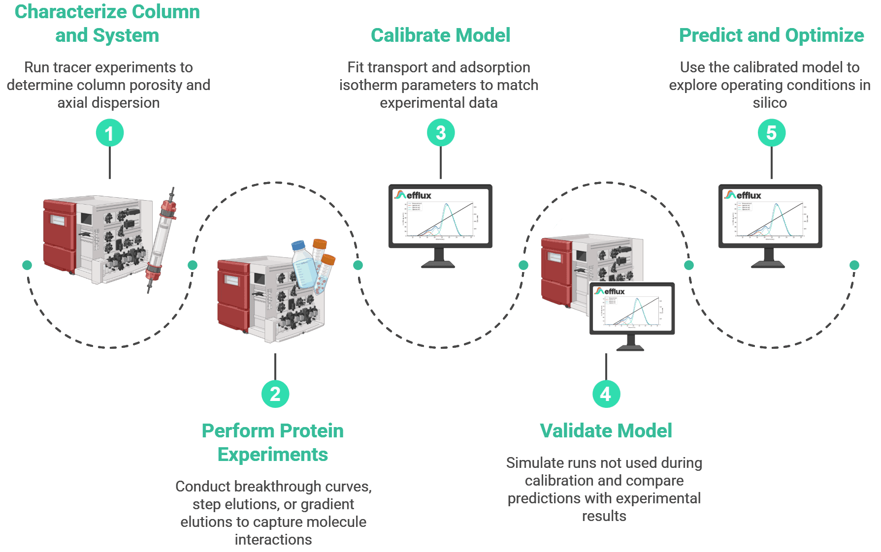
Once calibrated, the model is validated against 1–2 independent experiments that were not used during fitting. If the model predicts these with acceptable accuracy, it can be used predictively. This calibration effort is modest compared to a full DoE study (which typically requires 20-40 experiments), and unlike an empirical model, the calibrated mechanistic model can be reused across scales and conditions without re-running the experimental campaign.

What a Calibrated Model Enables

Because the model is rooted in physics, the transport and binding parameters do not change when the column diameter increases or the gradient profile is modified. An empirical model, by contrast, is only valid within the design space it was trained on.

In practice, a single calibrated mechanistic model can be used to:

• Screen thousands of operating conditions in silico — flow rates, gradient shapes, load densities, column dimensions
• Predict performance at manufacturing scale based on lab-scale data
• Evaluate the impact of lot-to-lot resin variability
• Assess process robustness and define proven acceptable ranges
• Establish design spaces for regulatory submissions within a QbD framework (ICH Q8, Q11)

Practical Considerations

Mechanistic modeling has been used in academic and industrial research for decades, but its adoption in routine process development has been slower. The main barriers have been software accessibility and the expertise required to set up, calibrate, and interpret the models.

This is changing. Cloud-based simulation platforms, such as Efflux, now provide structured workflows for model setup, calibration, and simulation, along with predefined templates for common column and system configurations. For teams without in-house modeling expertise, contract modeling services offer an alternative where the experimental work stays in-house while the modeling is handled externally.

The experimental requirements are also more manageable than they may appear. Standard pulse injections and step gradients (experiments that most process development labs already run) are often sufficient for calibration.