Getting Started with Mechanistic Modeling

Mechanistic modeling lets you predict chromatography performance from physical equations rather than trial and error. This page covers what you need to get started, the typical workflow, and how to decide when you have enough data to begin.

What You Need Before You Start

Before running a simulation you need information about your column and system, your molecules, and a small set of experimental data to calibrate the model against.

• Column and system information: Column dimensions (length and inner diameter), resin type, and particle diameter. Porosity values (total, interstitial, particle) are calculated from pulse injection experiments. You also need information about the physical setup around the column: tubing lengths and inner diameters, mixer volumes, and any other extra-column volumes that contribute to band broadening. Accounting for system dead volume is important for accurate simulations.
• Molecule properties: A rough estimate of molecular weight for each molecule in your system. If you are working with proteins, the amino acid sequence is enough to derive molecular weight and other useful properties like extinction coefficients.
• Experimental data: A small set of experimental chromatograms to calibrate the model against — typically pulse injections with a non-binding tracer to determine column transport parameters, and binding experiments (breakthrough curves, step elutions, or gradient elutions) to calibrate the adsorption isotherm. More detail is covered in Experimental Data.

The Modeling Workflow

Mechanistic chromatography modeling follows a structured workflow. Each step builds on the previous one.

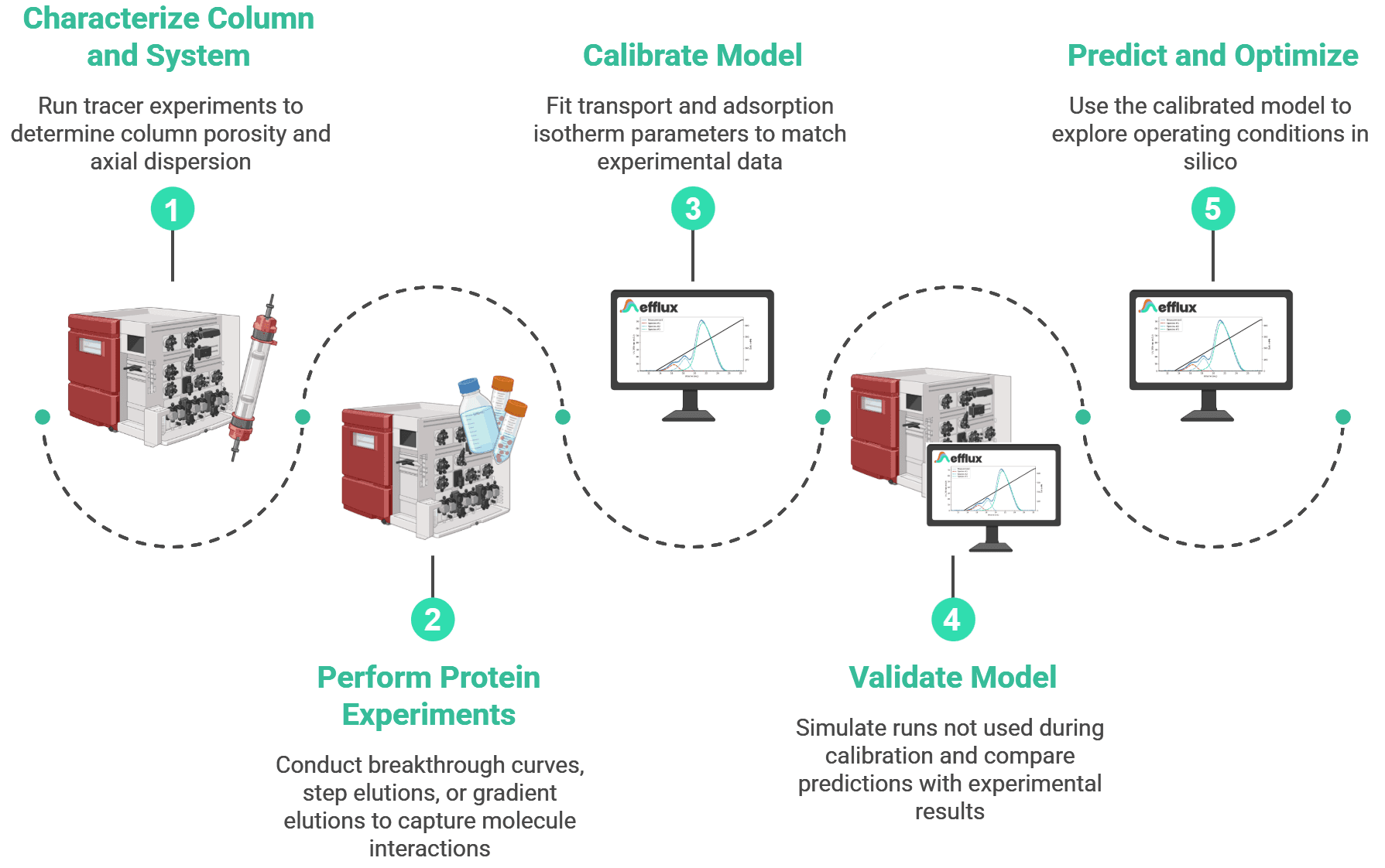
1. Characterize the column and system. Run non-binding tracer experiments (pulse injections) to determine column porosity and axial dispersion. At the same time, the system's extra-column contribution (tubing, mixers, dead volumes) is accounted for. These transport parameters are independent of the molecules you want to separate.
2. Perform protein experiments. Perform breakthrough curves, step elutions, or gradient elutions, that capture how your molecules interact with the stationary phase. These chromatograms serve as the calibration data for the model in the next step.
3. Calibrate the model. Using the experimental chromatograms from the previous step, fit the transport and adsorption isotherm parameters (e.g. equilibrium constants, maximum binding capacity, kinetic rates, diffusion coefficients, etc.) so that simulations match the experimental data.
4. Validate. Simulate runs that were not used during calibration and compare the predictions against experimental results. If the model predicts well under different conditions, it is ready for use.
5. Predict and optimize. Use the calibrated model to explore operating conditions in silico — screen gradient shapes, flow rates, loading conditions, or entirely different column formats without running additional lab experiments.

How Much Data is Enough?

One of the most common questions when getting started is how many experiments are needed. The answer depends on the complexity of your separation and the model you choose, but a few guidelines apply:

• Column and system characterization typically requires 2–3 pulse injections. This covers both column parameters and extra-column system effects. It is straightforward and usually takes less than a day of lab time, including preparation time.
• Model calibration is where most of the experimental effort goes. For a simple single-component system with a SMA isotherm, 6–10 experiments at different conditions (e.g. different load concentrations or gradient slopes) is usually sufficient.
• Validation needs at least 1–2 independent experiments. Conditions should differ from the calibration experiment set.

In practice, a simple single-column separation can be modeled from as few as 10 experiments total. This is significantly less than a traditional design of experiments (DOE) approach, which typically requires dozens of runs to cover the same design space.

Next Steps

With a basic understanding of what is needed, the next step depends on where you are in your workflow:

• If you need guidance on what experiments to run, see Experimental Data.
• If you want to understand the math behind the models, start with Mechanistic Modeling in the Scientific Background section.
• If you want step-by-step tutorials, the Guides section will walk through each step in detail.
• If you're ready to try it out, explore the Efflux simulator and book a demo.