Common Pitfalls and Best Practices
Mechanistic modeling is a powerful tool, but there are common mistakes that can lead to poor predictions or wasted effort. This page covers the pitfalls we see most often and how to avoid them.
Over-Parameterization
Over-parameterization is one of the most common mistakes in mechanistic modeling. It happens when you try to fit too many parameters at once relative to the amount of experimental data available. The optimizer finds a combination of parameter values that matches the calibration data well, but the parameters lose their physical meaning and the model fails to predict new conditions.
Signs that your model may be over-parameterized:
- Excellent calibration fit, poor validation: The model matches the training data almost perfectly but deviates significantly when predicting independent experiments.
- Physically unrealistic parameter values: Fitted values that are orders of magnitude away from expected ranges. For example, a diffusion coefficient that is 100x larger than what correlations predict.
- Parameter correlation: Two or more parameters compensate for each other, meaning you can change one if you also change the other without affecting the overall fit.
- Unstable fits: Running the optimizer with different starting values gives very different parameter estimates but similar fit quality.
To avoid over-parameterization:
- Fix parameters that can be measured or estimated independently (e.g. porosity from pulse injections, diffusion coefficients from correlations, tubing volumes from physical measuring) and only fit the parameters you truly cannot determine by other means.
- Calibrate in stages: Characterize column transport first, then fit binding parameters, rather than fitting everything simultaneously.
- Start with a simpler model and only increase complexity if the simpler model clearly cannot capture the observed behavior.
Model Selection
Choosing the right column model and binding model is a balance between accuracy and complexity. A more detailed model is not always a better model.
Column Models
The main column models differ in how they describe mass transfer within and around the resin particles. From simplest to most detailed:
- Lumped Rate Model (LRM): Combines all mass transfer resistances into a single lumped coefficient. Fast to solve and often sufficient for process optimization where exact peak shapes are less critical.
- Lumped Rate Model with Pores (LRMP): Distinguishes between film mass transfer (around the particle) and pore diffusion (inside the particle). A good balance between detail and computational cost for most applications.
- General Rate Model (GRM): Resolves the radial concentration profile inside each particle. The most accurate but also the most computationally expensive. Typically needed only when intra-particle gradients are significant, such as with large proteins or very fast flow rates.
Binding Models
The choice of binding model depends on the separation mode and the complexity of the interactions:
- Langmuir: The simplest nonlinear isotherm. Competitive multi-component binding with no salt modulation. Works well for affinity chromatography and simple separations where the modifier concentration does not influence binding. Three parameters per component (adsorption rate, desorption rate, and maximum capacity).
- MPM Langmuir: Mobile phase modulated Langmuir. Extends the Langmuir model with exponential and power-law salt dependence. A good middle ground when salt affects binding but the full SMA framework is not needed.
- Steric Mass Action (SMA): The standard choice for ion exchange chromatography. Models salt-dependent binding with steric shielding, where bound proteins block additional binding sites beyond what they physically occupy.
- HIC models (HIC 1, HIC 2): Specialized for hydrophobic interaction chromatography. HIC 1 models cooperative adsorption with salt-dependent desorption kinetics. HIC 2 adds competitive saturation and multi-factor modulation for more complex HIC systems.
- Colloidal 1: Models lateral interactions between adsorbed molecules on the surface. As surface coverage increases, the energy barrier for further adsorption rises. Useful when crowding effects on the resin surface are significant.
The general rule: use the simplest model that captures the behavior you observe. Each additional parameter requires more data to calibrate reliably and increases the risk of over-parameterization. See the Binding Models page for the full mathematical formulations.
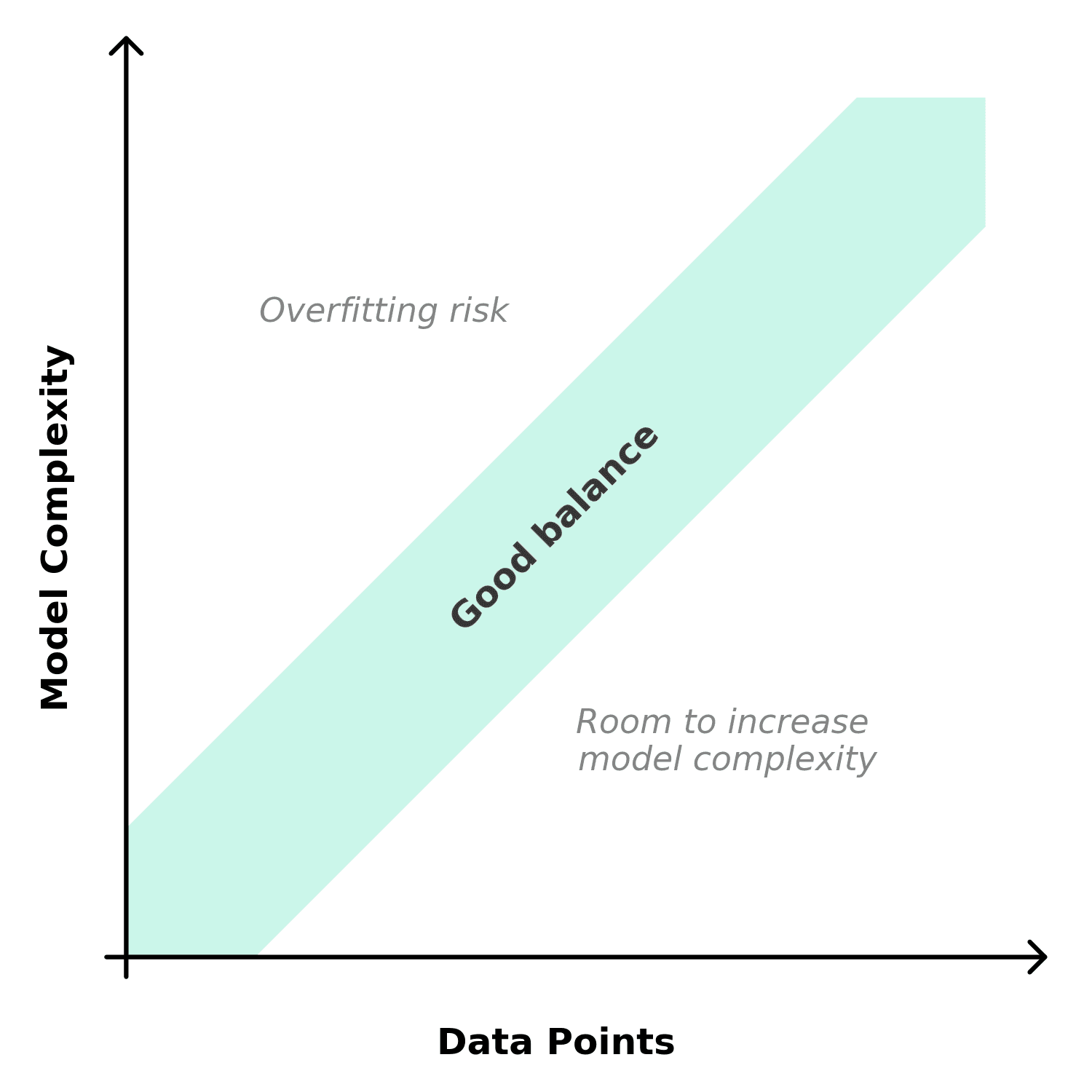
Matching Model Complexity to Available Data
The complexity of model you can reliably calibrate depends on how much experimental data you have. More parameters require more experiments to constrain them. If you do not have enough data, the optimizer will find parameter combinations that fit the calibration set but fail to predict new conditions.
Practical guidelines:
- If you only have 2–3 experiments, stick with simple models (LRM + Langmuir) and fit as few parameters as possible. Even then, with this few data points, you will most likely not be able to fit all parameters.
- If you have a well-designed dataset of 6–10 clean experiments at varied conditions, you can consider more detailed models (LRMP + SMA).
- If the model does not fit well despite having good data, the issue is more likely the choice of model (e.g. wrong binding mechanism) than the number of parameters.
When You Need More Data vs. a Different Model
When a model does not fit well to experimental data, it can be tempting to include more data. But more data only helps if the model is fundamentally capable of capturing the behavior. If it is not, more data just confirms that the model is wrong.
You likely need more data when:
- The model fits some experiments well but not others, and the poorly-fitted experiments are at conditions that are underrepresented in the calibration set (e.g. only one high-load experiment).
- Parameter estimates are unstable, different starting values give different results. More data helps constrain the parameters.
- You want to extrapolate to a regime that is far from your current data. A few bridge experiments at intermediate conditions can anchor the model.
You likely need a different model when:
- The model systematically misses a feature that is present in all experiments. For example, consistent peak tailing that the model predicts as symmetric, or an elution order that the model gets wrong.
- The fitted parameters are physically unrealistic despite having enough data. This suggests the model equations do not describe the actual mechanism.