Adsorption Isotherms in Chromatography

An adsorption isotherm describes the distribution of a protein between the liquid phase and the solid phase of the resin. In other words, it tells you how much protein is bound to the resin for a given concentration in the surrounding liquid. It determines how much a column can be loaded and how much salt or pH is needed to elute.

Adsorption isotherms in chromatography

Each point on an isotherm is an equilibrium between protein in the liquid at concentration $c$ and protein bound to the resin at concentration $q$. Most protein isotherms have the same basic shape. At low $c$, binding grows linearily with concentration. At high $c$, the resin runs out of free binding sites and $q$ levels off at the binding capacity. The Langmuir isotherm is the simplest equation that captures both:

where $q_{max}$ is the binding capacity and $K$ is the affinity of the protein for the resin. Other binding models differ mainly in how they get from the linear region to the plateau, and that difference can be large (Figure 1). Temperature is constant (hence "iso-therm").

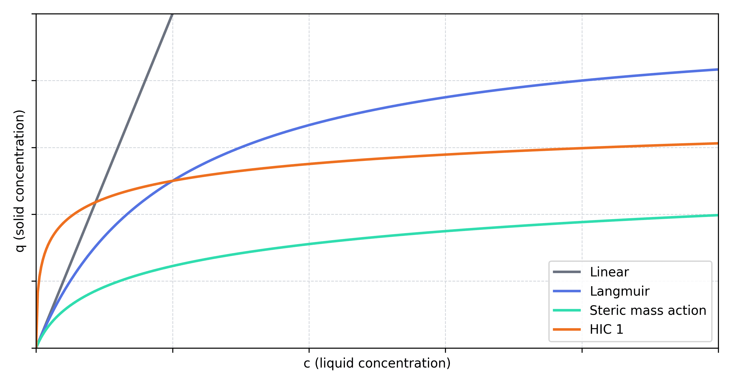
An isotherm that bends over and flattens out, like Langmuir, is called favorable. A linear isotherm, or one that curves upwards, is unfavorable. The difference shows up as soon as you load a column. With a favorable isotherm, high concentrations travel through the column faster than low ones, so the adsorption front stays sharp. With an unfavorable isotherm, the front spreads out as it moves down the column.

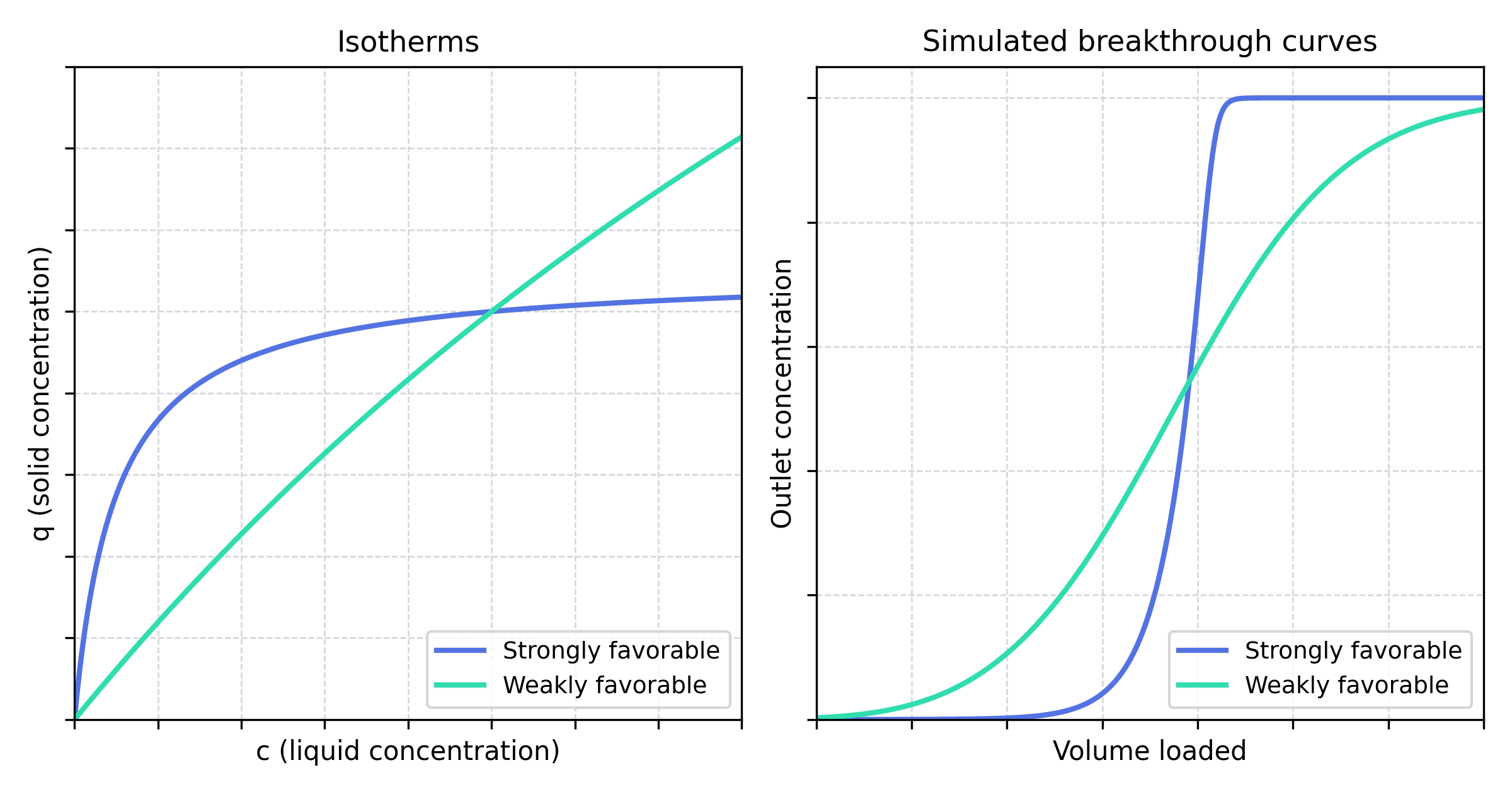
Figure 2 shows two isotherms that bind exactly the same amount at the feed concentration, simulated with Efflux on the same column. At saturation both columns hold the same amount of protein. The weakly favorable isotherm still breaks through much earlier, and the strongly favorable one takes about a third more feed before reaching 10% breakthrough. Static capacity alone doesn't tell you how much you can load.

The two Langmuir parameters control different parts of the curve. $K$ sets how steeply binding rises at low concentration, while $q_{max}$ sets where it levels off. A high-affinity protein saturates the resin at a low concentration. A low-affinity protein needs a much higher concentration to reach the same loading. Try changing both in Figure 3 below.

How does salt affect the isotherm?

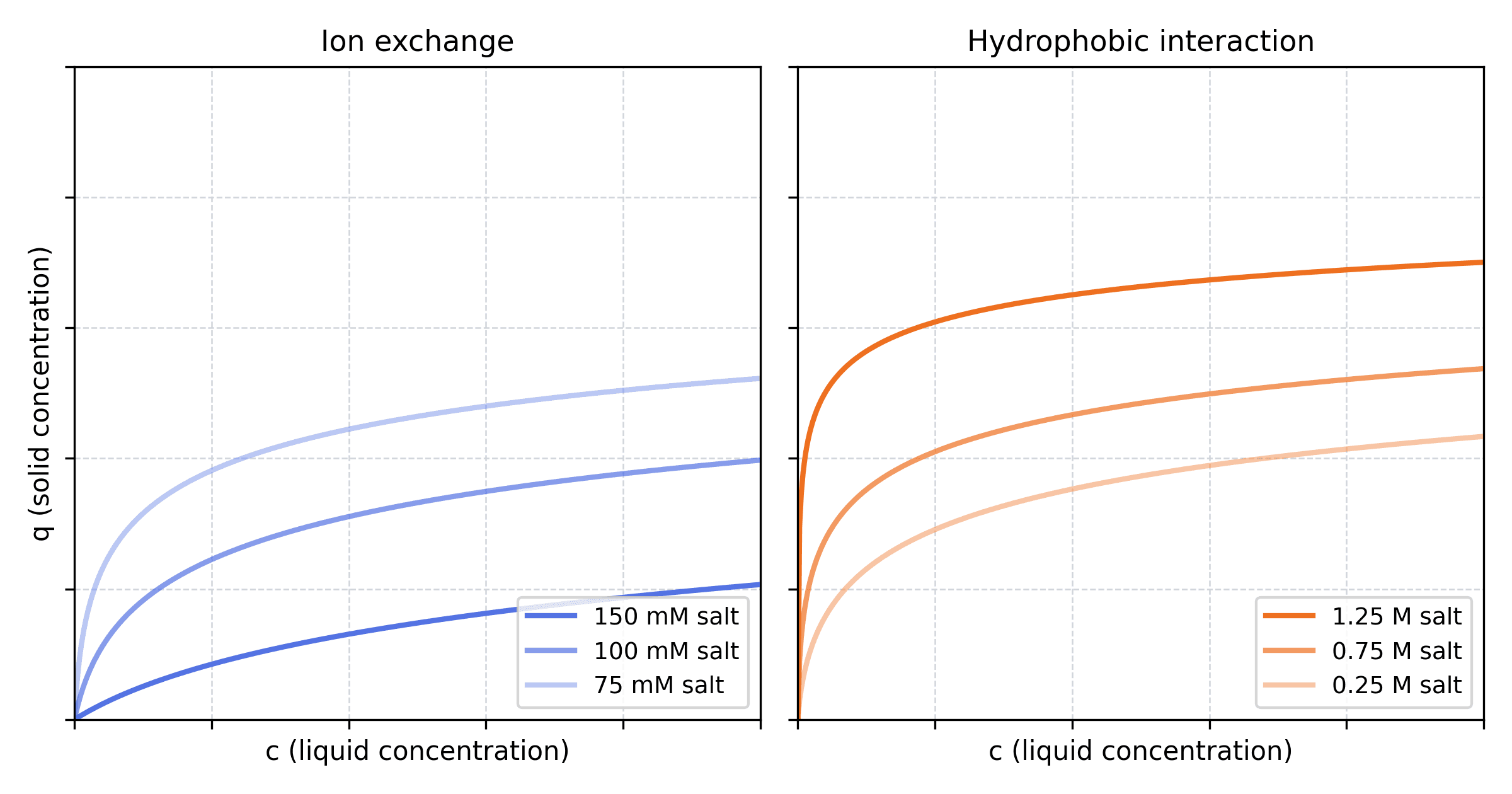
In ion exchange, salt ions compete with the protein for the charged sites on the resin, so more salt means less binding. The effect is steep. For a protein that binds through five charges, doubling the salt concentration lowers the initial slope of the isotherm by a factor of $2^5 = 32$. That's why a shallow gradient can still elute a tightly bound protein.

Hydrophobic interaction chromatography works the other way round. Kosmotropic salts such as ammonium sulfate strengthen hydrophobic binding, so binding increases with salt and you elute by lowering it (Figure 4). pH plays a similar role in ion exchange because it changes the protein's net charge.

How are adsorption isotherms determined experimentally?

The most direct method is a batch uptake experiment. Mix a known volume of resin with protein solution at a starting concentration $c_0$, wait for equilibrium (often several hours for large proteins), and measure what is left in the supernatant. A mass balance gives the bound concentration:

Each experiment gives one point on the curve, and you move along the curve by changing either the starting concentration or the resin volume. Changing the resin volume is usually easier, since it avoids preparing a dilution series. Running the series in 96-well filter plates makes it practical to cover several salt levels or pH values at once.

Cytiva's PreDictor isotherm plates can be used for this. They are 96-well filter plates prefilled with a ladder of resin volumes from 2 to 50 µL, so a single feed solution gives a complete isotherm. Measuring only the flowthrough and calculating $q$ from equation (2) avoids the extra error from washing and eluting the resin. A application note walks through examples for IgG on MabSelect SuRe and BSA on Capto Q at several salt concentrations.

Frontal analysis measures the same thing in a column. You pump feed through until it breaks through, and the area above the breakthrough curve, corrected for the hold-up volume, gives $q$. The linear region can also be estimated from retention times in pulse injections and linear gradient elution, which uses far less protein.

Adsorption isotherms in mechanistic modeling

A mechanistic model describes binding as a rate rather than an equilibrium. The Langmuir binding model, for example, is written as

where the first term is adsorption onto free sites and the second is desorption, with rate constants $k_a$ and $k_d$. At equilibrium the two terms cancel. Setting $dq/dt = 0$ gives back the isotherm in equation (1), with $K = k_a / k_d$.

Only the ratio of the rate constants appears in the isotherm. If binding is fast compared with mass transfer, your data will pin down $K$ well and say little about $k_a$ or $k_d$ on their own.

In practice the binding parameters are usually calibrated against chromatograms, not measured isotherms, so the isotherm is implied by the fit. Two binding models can match the same calibration run and still predict very different binding at a load you never tested. Calibrating across several loads and salt levels reduces that risk.

In Efflux, you can calibrate binding models against your own chromatograms and simulate runs at conditions you haven't tested.